In college, while learning genetics, you may be faced with data obtained from F1 and F2 generations of the crosses. And you are required to be able to recognize ratios in order to decide how many genes are involved, and whether or not epistasis (which we talked about last section) is taking place.
Example(1)
A cross between two pure-breeding white-fruited tomato plants produced and F1 generation which all plants had purple fruit. In the subsequent F2 generation 160 plants were obtained; of these 94 had purple fuit, and the rest had white fruit.
As we know nothing about the genes controlling fruit color in tomato, we must first ask ourselves a question: “DOES THE DATA FIT ANY OF THE KNOWN MENDELIAN RATIOS?”
Since only two phenotypes are involved, it can’t be 9:3:3:1, or 9:3:4 or any mendelian ratios with more than 2 numbers included.
On examination of ratios with 2 phenotypes, 9:7 looks like a possible candidate, but 3:1 may also fit.
- In this case, to decide which is the best to fit the data, we introduce a new approach to this problem: the Chi-square test.
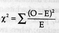
Chi-square(test)= sum[(obseved expected)ˆ2/expected]
(Xˆ2 is always calculated from original data, never from percentages, frequencies or proportions.)
- If Xˆ2 is large, the data doesn’t fit. A perfect fit gives Xˆ2 a zero. BUT HOW LARGE IS LARGE?
In addition to the result of Xˆ2, we need another piece of info to determine “how large is large”. We need to know the degrees of freedom.
Degrees of freedom are one less than the number of classes. They tell us something about the number of independent numbers we have, which relates to the usefulness of our data.
In this example, we have two phenotypic classes, purple, and white. It means when we have counted the purple ones, the number of the white ones is fixed so we have only one degree of freedom.
If we had three classes, we would have two degrees of freedom: when the two classes have been counted, the number of the third is fixed.
As the degrees of freedom gets bigger, Xˆ2 gets bigger. So the answer of HOW LARGE IS LARGE depends on different degrees of freedom.
- In this example, we determine which ratio is the best fit by comparing the value of Xˆ2
Observed result: 94 purple 66 white
Result predicted by 9:7 ratio 160×9/16 =90 160×7/16 =70
Xˆ2=[(94-90)ˆ2/90]+[(66-70)ˆ2/70]=0.41,with one degree of freedom
Result predicted by 3:1 ratio 160×3/4=120 160×1/4=40
Xˆ2=[(94-120)ˆ2/120]+[(66-40)ˆ2/40]=22.5,with one degree of freedom
- Using Xˆ2 probability tables can help quickly get to the value of Xˆ2.
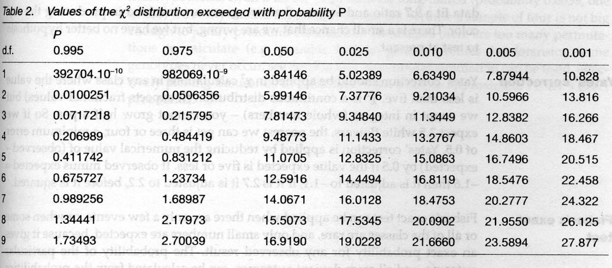
How to use it?
Follow the line for the one degree of freedom(top line) to find the nearest values of xˆ2 above and below our value.
We can see that the value of 0.41 is between the probability of 0.975 and 0.050 with an affinity to 0.975, which means that if we repeated the experiment 1000 times, we have a probability close to 97.5% that the observed ratio would fit 9:7. The value of 22.5 is way beyond way exceeded with the probability of 0.001, which suggests that 3:1 ratio doesn’t fit the data.
====================================================
Data analysis after class:
A cross between pure-breeding white-fruited and purple-fruited tomato plants produced and F1 generation which all plants had purple fruit. In the subsequent F2 generation 160 plants were obtained; of these 99 had purple fuit, 25 had red fruit, and 36 had white fruit.
====================================================
卡方检验是以χ2分布为基础的一种常用假设检验方法,它的无效假设H0是:观察频数与期望频数没有差别。

该检验的基本思想是:首先假设H0成立,基于此前提计算出χ2值,它表示观察值与理论值之间的偏离程度。根据χ2分布及自由度可以确定在H0假设成立的情况下获得当前统计量及更极端情况的概率P。如果P值很小,说明观察值与理论值偏离程度太大,应当拒绝无效假设,表示比较资料之间有显著差异;否则就不能拒绝无效假设,尚不能认为样本所代表的实际情况和理论假设有差别。